Why vectorize?

I recently found myself having to compute a large set of performance metrics for training my deep learning models. These metrics included Spearman correlation and auPRC—specifically, how well do the predictions align with the true values, and how good the precision and recall are. Unfortunately, these metrics needed to be computed separately for up to millions of data points (i.e. each data point is a vector, and correlation/auPRC needed to be computed over each vector). That is the nature of computational biology, I suppose. C’est la vie.

What is even more unfortunate is that NumPy, SciPy, and Sklearn don’t have vectorized implementations for most of these metrics. This is hardly surprising, because Spearman correlation and auPRC both require special treatment of “ties” in the data.

That said, I simply could not stand the time it took to compute these metrics by calling NumPy/SciPy/Sklearn functions one at a time (even parallelized across threads). Thus, I’ve implemented vectorized versions of these functions.

The code for vectorized correlation and auPRC can be found below, or in this GitHub repository

Below, I’ll briefly describe the way these functions can be vectorized, including the nifty little tricks that can be done.

Benchmarking

To benchmark the vectorized code compared to the unvectorized library functions, I synthesized many random vectors of length 1000, and computed Spearman correlation or auPRC using two methods: 1) calling the vectorized functions, which compute over the entire matrix at once; and 2) calling the library functions one by one in a for loop. The results are as follows:

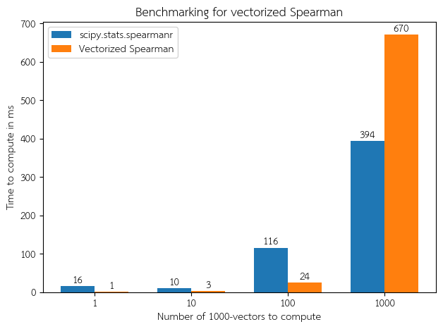
Note that once the number of vectors gets too large, the benefit of vectorization is completely masked by the penalty caused by excess swapping/paging. For large inputs, I recommend batching into smaller chunks. This would take advantage of vectorization maximally while not impinging a memory penalty.

How to vectorize Spearman correlation

Spearman correlation is defined as the Pearson correlation of the ranks of data in the input vectors. If all the entries in the vectors were unique, then this would be a very easy task to vectorize, since np.argsort can effectively compute ranks in a vectorized way; furthermore, Pearson correlation is easily vectorized, since it’s simply a ratio of empirical expectations. The difficulty in vectorizing Spearman correlation is when there are ties in the data. Traditionally (and this is how scipy.stats.spearmanr does it), ties in the input vectors are assigned the average rank. While SciPy does provide a scipy.stats.rankdata function that ranks data by using averages for ties, it is not vectorized. This involves interrogating the set of unique elements in each vector. To do this in a vectorized fashion is difficult, but fortunately, there is a nasty little trick we can use!

First off, it’s easy to compute Pearson correlation in a vectorized way.

def pearson_corr(arr1, arr2):
    """
    Computes Pearson correlation along the last dimension of two multidimensional arrays.
    """
    mean1 = np.mean(arr1, axis=-1, keepdims=True)
    mean2 = np.mean(arr2, axis=-1, keepdims=True)
    dev1, dev2 = arr1 - mean1, arr2 - mean2
    sqdev1, sqdev2 = np.square(dev1), np.square(dev2)
    numer = np.sum(dev1 * dev2, axis=-1)  # Covariance
    var1, var2 = np.sum(sqdev1, axis=-1), np.sum(sqdev2, axis=-1)  # Variances
    denom = np.sqrt(var1 * var2)

    # Divide numerator by denominator, but use NaN where the denominator is 0
    return np.divide(
        numer, denom, out=np.full_like(numer, np.nan), where=(denom != 0)
    )

Now let’s compute the average ranks of a data in a vectorized way. First, we generate the ranks for each vector, with the ties broken arbitrarily. In this step, we sort the input array based on the indices, and then assign each element a rank.

def average_ranks(arr):
    """
    Computes the ranks of the elements of the given array along the last dimension.
    For ties, the ranks are _averaged_. Returns an array of the same dimension of `arr`. 
    """
    sorted_inds = np.argsort(arr, axis=-1)  # Sorted indices
    ranks, ranges = np.empty_like(arr), np.empty_like(arr)
    ranges = np.tile(np.arange(arr.shape[-1]), arr.shape[:-1] + (1,))

    np.put_along_axis(ranks, sorted_inds, ranges, -1)
    ranks = ranks.astype(int)

Next, we create an array where each entry maps a unique element in the original array to a unique index for that vector. To do this, we take the sorted vectors and take pairwise difference. Whenever the difference is 0, there is a run of identical elements. Whenever the difference is not 0, the two elements on either side are unique. We turn these nonzero entries into 1, so when we take the cumulative sum, we get unique_inds. The entries of unique_inds are indices, where the location of the index in unique_inds is the end of a “run” of non-unique elements in the sorted vectors, and the value of the index is the index of the unique entries. This means that for a vector, the number of unique indices in unique_inds is the number of unique elements in the original vector.

    sorted_arr = np.take_along_axis(arr, sorted_inds, axis=-1)
    diffs = np.diff(sorted_arr, axis=-1)
    # Pad with an extra zero at the beginning of every subarray
    pad_diffs = np.pad(diffs, ([(0, 0)] * (diffs.ndim - 1)) + [(1, 0)])
    # Wherever the diff is not 0, assign a value of 1; this gives a set of small indices
    # for each set of unique values in the sorted array after taking a cumulative sum
    pad_diffs[pad_diffs != 0] = 1
    unique_inds = np.cumsum(pad_diffs, axis=-1).astype(int)

Now, we can compute average ranks. We use the indices in unique_inds index into an array that stores the average of the ranks of the groups of unique elements in the original vectors. We take advantage of the fact that np.put_along_axis will clobber earlier entries with later ones if the same destination index is specified multiple times. Note that unique_maxes will have empty spots if there are repeat elements in a vector, and we will only use the whole vector in unique_maxes if the original vector had all unique entries. Once we have the maximum rank of each set of unique entries in unique_maxes, we can easily compute the average ranks by taking pairwise differences and doing some clever algebra. unique_avgs holds these average ranks, one for each set of unique elements in the original vector.

    unique_maxes = np.zeros_like(arr)  # Maximum ranks for each unique index
    # Using `put_along_axis` will put the _last_ thing seen in `ranges`, which will result
    # in putting the maximum rank in each unique location
    np.put_along_axis(unique_maxes, unique_inds, ranges, -1)
    # We can compute the average rank for each bucket (from the maximum rank for each bucket)
    # using some algebraic manipulation
    diff = np.diff(unique_maxes, prepend=-1, axis=-1)  # Note: prepend -1!
    unique_avgs = unique_maxes - ((diff - 1) / 2)

Finally, we assign the average ranks to the elements of the original vector. Note that when there are ties in the original vector, all elements that have the same value get the same average rank.

    avg_ranks = np.take_along_axis(
        unique_avgs, np.take_along_axis(unique_inds, ranks, -1), -1
    )
    return avg_ranks

Finally, to compute Spearman correlation, we simply compute the average ranks of both inputs, and calculate the Pearson correlation.

How to vectorize auPRC

Computing auPRC is a bit tricky, because it’s important to implement it the “right” way. Sklearn currently has two methods of computing auPRC, but the “correct” way to do so is implemented by the sklearn.metrics.average_precision_score function. Specifically, this function estimates auPRC by computing recall and precision for different “buckets”, based on different thresholds in the predicted values. Importantly, this function will use bucket thresholds that are the unique entries of the predicted values. This thresholding is nuanced, but critical.

To compute auPRC, we first sort the predicted values in descending order (to eventually get the thresholds/buckets to compute precision and recall), and sort the true values correspondingly.

def auprc_score(true_vals, pred_vals):
    """
    Computes the auPRC in the last dimension of `arr1` and `arr2`. `true_vals` should contain
    binary values; any values other than 0 or 1 will be ignored when computing auPRC.
    `pred_vals` should contain prediction values in the range [0, 1].
    If there are no true positives, the auPRC returned will be NaN.
    """
    sorted_inds = np.flip(np.argsort(pred_vals, axis=-1), axis=-1)
    pred_vals = np.take_along_axis(pred_vals, sorted_inds, -1)
    true_vals = np.take_along_axis(true_vals, sorted_inds, -1)

Next, we compute the indices where a run of identical predicted values ends. We create the array thresh_inds, which contains a 1 wherever a run ends, and 0 otherwise. We also create a boolean mask version of this array, thresh_mask.

    diff = np.diff(pred_vals, axis=-1)
    diff[diff != 0] = 1  # Assign 1 to every nonzero diff
    thresh_inds = np.pad(
        diff, ([(0, 0)] * (diff.ndim - 1)) + [(0, 1)], constant_values=1
    ).astype(int)
    thresh_mask = thresh_inds == 1

Now, we compute the number of true positives and false positives were we to threshold at each possible location. Note that this will compute the true/false positives at every possible threshold, not just the places where the runs end. We will ignore these extraneous entries later. At the same time, we take this opportunity to mask out anything in the true values that was not 0 or 1. This can be useful if there are “ambiguous” values in the true values that we wish to ignore when computing auPRC.

    weight_mask = (true_vals == 0) | (true_vals == 1)
    true_pos = np.cumsum(true_vals * weight_mask, axis=-1)
    false_pos = np.cumsum((1 - true_vals) * weight_mask, axis=-1)

Next, we compute precision and recall. When we compute precision, we keep a 0 wherever there is not a threshold we want to consider (i.e. put a 0 wherever there isn’t an end of a run), and where the precision is not defined. For recall, we put NaN wherever it is not defined. In particular, if there are no true positives, then the recall is NaN for that entire vector.

    precis_denom = true_pos + false_pos
    precis = np.divide(
        true_pos, precis_denom,
        out=np.zeros(true_pos.shape),
        where=((precis_denom != 0) & thresh_mask)
    )
    recall_denom = true_pos[..., -1:]
    recall = np.divide(
        true_pos, recall_denom,
        out=np.full(true_pos.shape, np.nan),
        where=(recall_denom != 0)
    )

Next, we do some padding to make sure the first bucket is computed properly.

    # Concatenate an initial value of 0 for recall; adjust `thresh_inds`, too
    thresh_inds = np.pad(
        thresh_inds, ([(0, 0)] * (thresh_inds.ndim - 1)) + [(1, 0)],
        constant_values=1
    )
    recall = np.pad(
        recall, ([(0, 0)] * (recall.ndim - 1)) + [(1, 0)], constant_values=0
    )
    # Concatenate an initial value of 1 for precision; technically, this initial value won't
    # be used for auPRC calculation, but it will be easier for later steps to do this anyway
    precis = np.pad(
        precis, ([(0, 0)] * (precis.ndim - 1)) + [(1, 0)], constant_values=1
    )

Now we compute the difference of the recalls, but only in buckets marked by the threshold indices in thresh_inds. Since the number of buckets can be different for each vector, we create a set of bucketed recalls and precisions for each bucket. This is a similar trick to the one used to compute unique ranks in Spearman correlation above. Each entry in thresh_buckets is an index mapping the thresholds themselves to indices of consecutive buckets in recall_buckets and precis_buckets.

    thresh_buckets = np.cumsum(thresh_inds, axis=-1) - 1
    # Set unused buckets to -1; won't happen if there are no unused buckets
    thresh_buckets[thresh_inds == 0] = -1
    # Place the recall values into the buckets into consecutive locations; any unused
    # recall values get placed (and may clobber) the last index
    recall_buckets = np.zeros_like(recall)
    np.put_along_axis(recall_buckets, thresh_buckets, recall, -1)
    # Do the same for precision
    precis_buckets = np.zeros_like(precis)
    np.put_along_axis(precis_buckets, thresh_buckets, precis, -1)

Finally, now that the entries in recall_buckets and precis_buckets are recall and precision values for only the bucket thresholds, and they are contiguous in these arrays, we can compute the area under the precision-recall curve using np.diff.

    # Note that when `precis` was made, it is 0 wherever there is no threshold index,
    # so all locations in `precis_buckets` which aren't used (even the last index) have a 0
    recall_diffs = np.diff(recall_buckets, axis=-1)
    return np.sum(recall_diffs * precis_buckets[..., 1:], axis=-1)