Neural networks are really good at learning how to map from a high-dimensional input to some output prediction. This constitutes the core idea behind supervised learning (i.e. learn how to transform an input—like an image—into a known label—like whether the image contains a cat or a dog). In an unsupervised setting, a neural network is trained to represent the distribution of inputs in a latent space of smaller dimensionality. This is typically done without any guidance to the network, which learns latent-state representations completely independent of pre-existing knowledge.

As we’ll see below, this can lead to some very uninterpretable latent states, which can run contrary to our expectations. Instead of letting the unsupervised algorithm roam free, we may impose structure into the learned latent space, based on our pre-existing understanding of the dataset. Here, I’ll be showing a brief foray (using the MNIST dataset) into how we might improve the interpretability of the latent state by imposing our knowledge of distinct classes between the inputs.

Autoencoders

An autoencoder (AE) is one of the most common ways to learn the latent space of a set of inputs in an unsupervised way. It is trained on a set of input data points, and learns to reproduce the input as closely as possible as the output. An autoencoder consists of an encoder, \(E\), and a decoder, \(D\) where both are learned as neural networks. The encoder \(E\) learns to project an input \(x\) into a vector in the latent space, \(E(x) = h\), where \(h\) is of significantly lower dimensionality than \(x\). The decoder \(D\) is trained to recover \(x\) as much as possible from \(h\).

Typically, an AE is trained to minimize the discrepancy between \(x\) and \(D(E(x))\). Effectively, it learns a representation of the training distribution in the latent space. The main motivations/benefits of an AE are that it can be used to: 1) reduce the number of features required to represent an input distribution (e.g. for efficient storage); 2) identify the features most important for preserving variability of the input space; 3) sample latent vectors from the latent space to generate novel objects drawn from the input distribution; and 4) perform latent-space optimization to generate examples matching a particular archetype.

An uninterpretable latent-space landscape

On their own, AEs learn latent-space representations that are driven solely by isolating and projecting the most variable features in the input data. This, however, neglects any structure in the input distribution other than the most variable features. This can lead to the AE’s learning a latent-state representation that is not interpretable to humans, and can result in decoded outputs that go against human intuition, particularly when the dimensionality of the latent space is low.

Here’s an example of what happens if we train an AE on MNIST. If we plot a few random digits and their reconstructions, we see there’s a good amount of confusion between the digits. We’ll limit ourselves to latent spaces of dimension 1 or 2 only, to really show what’s going on. AEs with very limited latent-space dimensionalities are also often very desirable, as they dramatically condense the space required to represent an object, and substantially boost reliance on the most important features describing the input distribution.

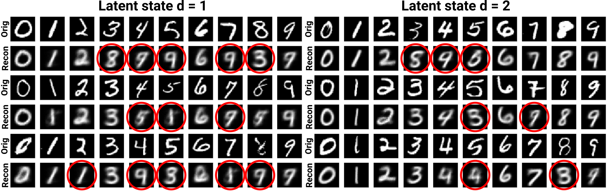
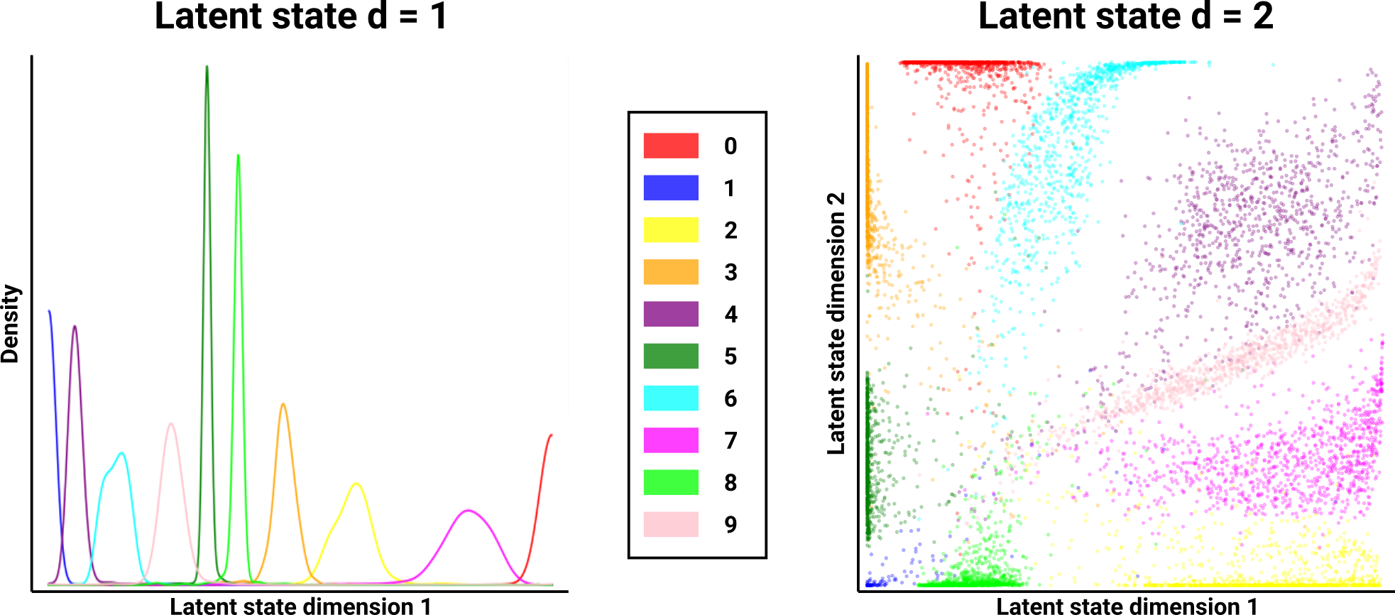
Although the network is trying its best to reconstruct the original input \(x\) using \(D(E(x))\), it is frequently mixing up digits like 4s and 9s. 3s and 8s also seem to be problematic. This contradicts our expectation as humans that digits like 4 and 9 are completely separate classes. The problem is that the network has no idea that 4s and 9s are supposed to be different classes. These digits look very similar already, and so the AE just learns them as one concept. We can further see just how badly the AE is conflating different digits by examining how the different representations \(h\) are distributed for each digit in the latent space. Note that since we restricted ourselves to just 1 or 2 dimensions in the latent space, this is easy to plot:

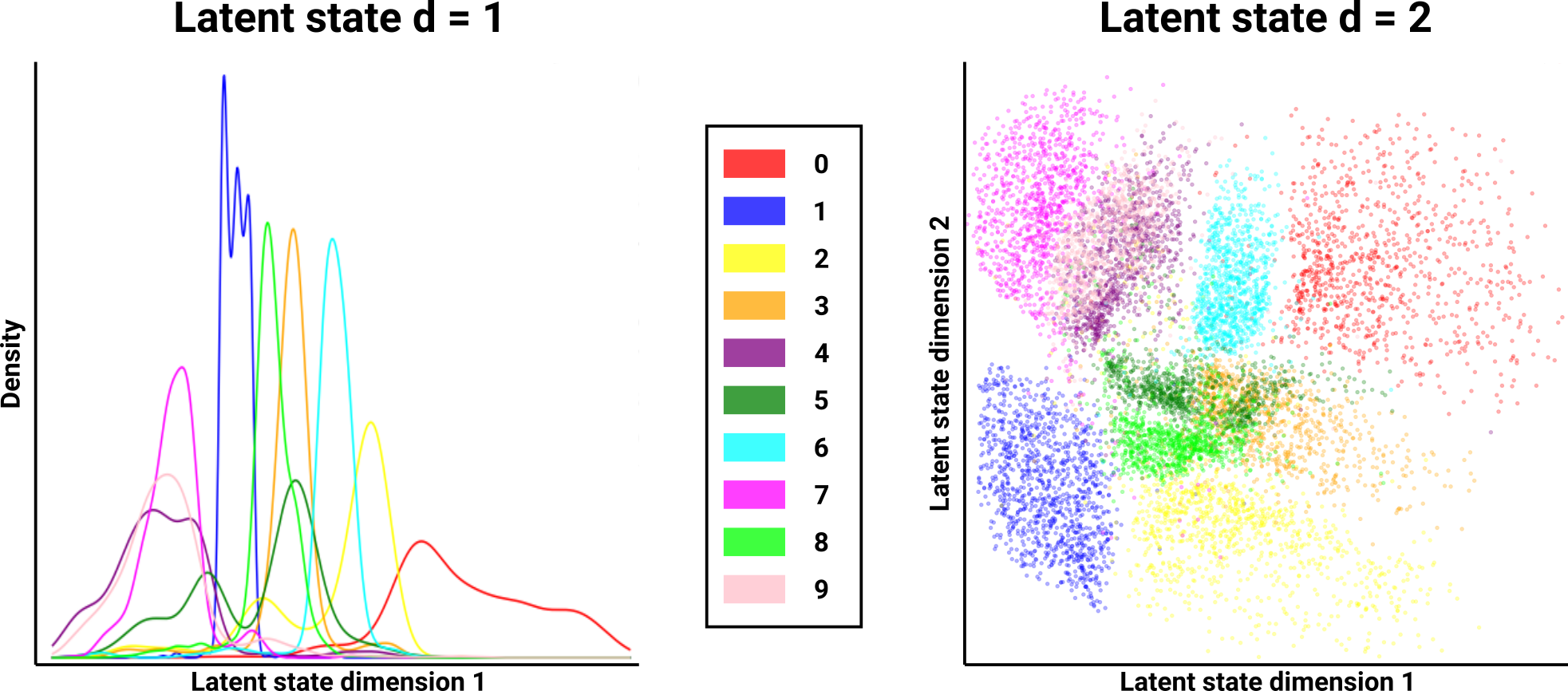
It’s no surprise that our AEs are having so much trouble reconstructing numbers in a way that respects the distinct digits. The latent space is a mess. In the case of 1 dimension, the AE learns how to project an input image into a single scalar, and reconstructs the original digit as best it can. We can see that numbers like 4, 7, and 9 share nearly an identical distribution of latent states. 3, 5, and 8 also overlap significantly. Note that because the AE reconstructs a digit solely from \(h\), if the distributions of distinct digits overlap, there is no way for the network to distinguish the two digits. In the 2-dimensional case, there is still a huge amount of overlap between 4 and 9, as well as between 3, 5, and 8. This illustrates how the AE fails to learn distinct representations for different digits, which leads to reconstructions that seem clearly wrong to us humans. Additionally, because the latent-space distributions are so similar between different digit classes, it is extremely difficult to use these AEs to generate novel digits of a desired class. For example, it is challenging to draw a latent-state sample that generates a 4, but not a 9. The concept of a 4 and a 9 are fundamentally different in our eyes, and perhaps a network trying to learn a latent representation of these digits should know that, as well.

Imposing class structure to the latent space

In order to improve the interpretability and subsequent usefulness of the AE, we can impose structure on the learned latent state, informed by external domain knowledge. For example, if the input distribution contains several different classes of inputs (e.g. MNIST naturally contains 10 different classes for the digits; CIFAR contains labels for the different classes of objects in the images), then we would expect the latent state to reflect this structure. As humans, we consider the different digits to be distinct, and so we reason about them separately. Similarly, it would be desirable for the encoder \(E\) to be interpretable in the same way, mapping all inputs of a particular class to a subregion of the latent space that is largely disjoint from all other classes. Ideally, any overlaps would only be for individual examples that are truly ambiguous (e.g. if someone were to write a digit whose identity is ambiguous even for a human).

For example, if we were to train an AE on MNIST, we would want to be able to generate novel examples of a 4 or a 9, and not a hybrid of the two that does not correspond to anything in the input distribution. As humans, 4s and 9s are completely distinct concepts in our mind. In turn, structuring the latent space so that the latent-state representations of 4s and 9s are disjoint can be extremely helpful, as it encourages the network to learn about 4s and 9s separately, which is what humans care about most of the time. By incorporating domain knowledge and structure into the latent space, an AE can be trained such that the latent states are far more interpretable. Subsequently, this could: 1) improve the quality of generated objects; 2) make it easier to generate novel objects of a specific class or archetype within the input distribution; and 3) allow us to leverage far more training data by letting the AE learn different latent-space distributions for different kinds of inputs.

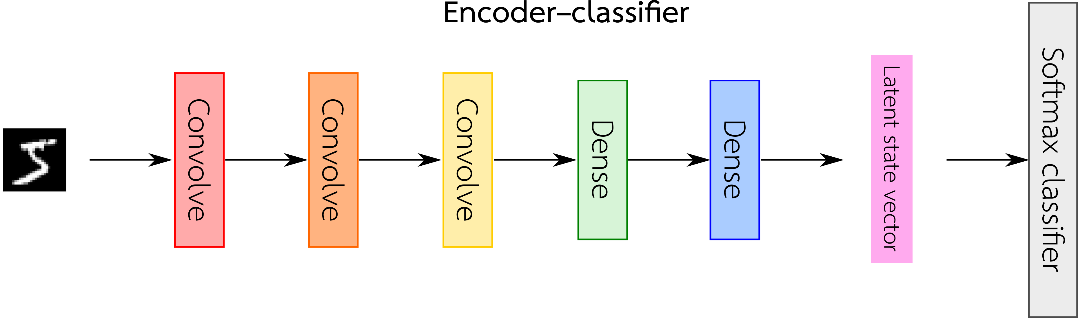
In order to impose class structure onto the learned latent space, we train the same AE architecture, but with a pretraining step in which the encoder \(E\) is first trained to be a classifier. That is, prior to training the AE, we train only the encoder portion as an MNIST classifier (i.e. an “encoder–classifier”) by adding on a few extra dense layers and a softmax output. Importantly, these dense layers operate on each digit class separately, so that the range of the latent space may be partitioned into disjoint regions for each digit class. After pretraining, we then remove the added dense layers and fine-tune the decoder (i.e. by freezing the encoder weights), and then fine-tune the entire AE as a whole.

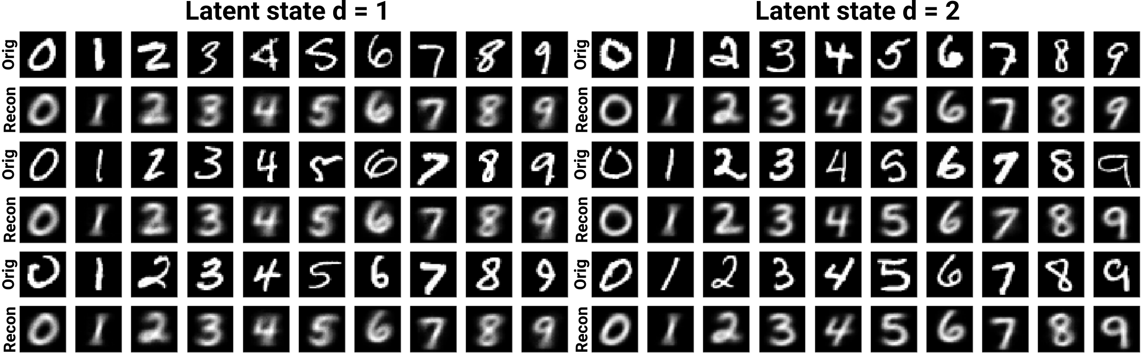
Pretraining the encoder to be a classifier implicitly encourages it to keep the latent-state representations disjoint between digit classes. Upon fine-tuning the AE as a whole, the latent states show much cleaner distributions that are separate from each other. That is, the latent space is far more interpretable, where we can easily partition it into distinct subregions that represent each digit. Subsequently, this results in reconstructed digits that are no longer conflated between different digit classes. Furthermore, this makes generating novel digits of a specific class much more straightforward, as a latent-state vector can be sampled from a single digit class’ distribution, which more confidently does not encode a digit from any other digit class. Notably, although the distribution of latent-state representations are now more disjoint between the different digits, they still cluster together based on similarity as before (e.g. 4s and 9s are still closer together than the other digits).

Other forms of latent-state priors

Encoder–regressors: Disjoint classes are not the only way in which an input distribution can be structured. For a dataset like MNIST, the digits form very natural classes which our AE would hopefully encode as disjoint (or close to disjoint) latent-space distributions. Another way that input distributions can be structured, however, is by ordering or by relative magnitude. For example, on an AE that generates images of people’s faces, we may find it important (depending on the application) to order images based on attributes such as skin tone (dark to light) or face shape (thin to full). Subsequently, we would want the AE to learn this ordering as part of its latent-space representations. In this example, this may help the AE avoid generating faces of the wrong ethnicity or shape, and may aid in the generation of novel faces of a specific desired type. To pretrain the encoder, a single dense layer (of 1 or more outputs for 1 or more regressive tasks) with no nonlinearity can be added to the encoder, and the resulting encoder–regressor is trained (e.g. to predict skin tone or face shape).

Latent-state prior loss functions: In the MNIST example above, we pretrained the encoder as a classifier to induce the latent-state representations to be largely disjoint between the classes. Pretraining acted as a way to “inject” our prior knowledge of the digit classes into the AE. An alternative way to introduce this prior is by training with a secondary loss function (without any pretraining). For example, at training time, this secondary “latent-state prior” loss could consider the classes of the various inputs in the training batch, and penalize the model based on the latent states: the model is penalized for small Euclidean distances or cosine similarities between latent states of inputs belonging to different classes. For regressive structures, a different latent-state prior loss can be used. For example, at training time, this loss could compute the pairwise cosine similarities between the latent states of the inputs, and the model can be penalized if these similarities do not have a high Pearson correlation with the ordering of the inputs.

Caveats

As mentioned above, this is really only a brief proof of concept (as well as a kind of cool thing to show), and so there are a few caveats:

• To apply this idea of imposing class structure onto the latent space more broadly, we would want to titrate between how much information is learned from the imposed structure, and how much of the latent space is learned in a truly unsupervised manner; in the extreme, if the structure we impose is too strong, the autoencoder may ignore any inherent hidden structure in the latent space we want it to learn
• There seems to be a tradeoff between how disjoint we can get the latent-space representations for the different classes, and the variability in the representations within each class
• I only examined very low latent-space dimensionalities

I’d be happy to share source code and more detailed methods to anyone who would like; just contact me.