Disclaimer: This post is not meant to be a comprehensive overview; rather, it is my own thoughts and perspectives in paragraph form

With their high expressivity and capacity, neural networks have proven to be exceptional at fitting to complex datasets. They are able to learn functions mapping images to their English descriptions, users to their preferred advertisements, DNA sequences to their functions, etc. The list goes on. After all, the universal approximation theorem shows that a sufficiently wide and deep feed-forward neural network can represent any function whatsover. Unfortunately, despite their celebrated success on the surface, these models often struggle to fit to datasets and can fail in spectacular ways:

1) Failure to fit to data

A neural network might completely fail to capture the complexity of the data or produce a meaningful output. Most machine-learning researchers can likely recall lamenting at a neural network which has failed to achieve significantly better-than-random performance, despite a clear learnable signal being present in the dataset.

2) Poor generalization

Even if a neural network predicts correct outputs on the training set, a model might fail to generalize to the test set or new datasets outside of the study. This is another failure mode that most (if not all) machine-learning researchers have encountered.

3) Improper decision rules

A neural network that seems to perform well and generalizes to the test set might still be relying on improper or undesirable decision rules. Many models learn to make decisions based on noise, dataset-specific signals, or other features that simply should not be used. Unfortunately, this failure mode is not considered as often, as many reseachers and engineers tend to evaluate models solely based on performance without considering the reason why the decisions are made as they are. This failure mode, however, can still have devastating effects that go unnoticed until the model is deployed on data that does not exactly match the exact training/test distribution. For example, many neural networks trained to predict cancer images can easily learn to make decisions based on which CT machine generated the image (1). There are also countless horrifying examples of neural networks which learn to make decisions for extremely racist reasons (2) (3).

Hypotheses and the loss landscape

For simplicity, let us consider a binary classification setting, where some machine-learning model is trained to predict inputs as being positives or negatives.

Let \(P\) be the space of all possible inputs (e.g. for 100 x 100 grayscale images, \(\vert P \vert = 256^{100\times 100}\)). In some problems, \(P\) may even be infinite. A trained model will learn a function which takes in any input \(p \in P\) and outputs if it is a positive or a negative. We can represent this learned function as a hypothesis, \(h\). We define \(h\) to be the set of all points which the model predicts is positive (e.g. a typical binary classification model \(f\) with a sigmoid output would correspond to a hypothesis \(h = \lbrace p : f(p) > 0.5\rbrace\)). Let \(H\) be the set of all possible hypotheses \(h\). Note that in the binary classification setting, \(H\) is the powerset of \(P\), and \(\vert H\vert = 2^{\vert P\vert}\). That’s a lot of hypotheses to consider, and when we train our models, we are hoping that the final hypothesis we pick out of \(H\) is a good one.

What defines a good model (i.e. hypothesis) from a bad one? We define a risk \(R(h)\), which is the probability that the classifier with hypothesis \(h\) misclassifies a randomly drawn point from \(P\). Importantly, there is some distribution over \(P\) which defines how likely each point in \(P\) will occur. A classifier \(h^{*}\) that achieves the minimal possible risk \(R(h^{*})\) is the most optimal classifier that could exist.

Note that our analysis of \(H\) was simplified by assuming a binary classification task, but easily extends to other settings, where \(H\) and \(R\) grow in complexity.

Unfortunately, since we only have access to a limited number of points (a small subset \(\hat{P} \subset P\)), we cannot consider the minimization of \(R(h)\) directly, so instead we attempt to minimize the empirical risk \(\hat{R}(h)\), which is the probability \(h\) mispredicts a randomly drawn point from \(\hat{P}\). Notably, it is computationally intractable to even minimize \(\hat{R}(h)\) in general (\(H\) is simply too large to try every possible hypothesis \(h\)) and so different machine learning algorithms use different methods to approximate this minimization.

For neural networks, \(\hat{R}(h)\) is approximately minimized using some form of the gradient-descent algorithm. We define a loss function \(L\) which is meant to approximate \(\hat{R}\), and we pretend that the highly non-convex loss landscape is actually convex, and follow the gradients downhill until we reach a good local minimum which hopefully corresponds to a good model.

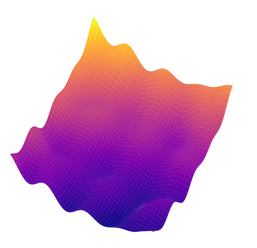
The image above shows a cartoon depiction of a simple loss landscape, for a model which only has 2 parameters. Depending on where we start in the random initialization of these parameters, we could end up in any one of many local minima. Each local minimum corresponds to a different instantiation of the model’s parameters (equivalently, a different hypothesis).

By optimizing over our loss landscape, we hope to minimize \(\hat{R}(h)\), which we hope also minimizes \(R(h)\). The reason we run into the challenges above (failure to fit, generalize, or learn proper decision rules) is that the local minimum we find in the loss landscape often does not actually correspond to a small \(R(h)\).

As an aside, it’s worth pointing out that if we had the optimal model that minimizes \(R(h)\), then there would be less of a need to verify that the model has learned “proper” decision rules. Of course, having a model which bases its decisions on human-interpretable rules has its avantages regardless (e.g. for humans to learn something about the world from these models). From the standpoint of wanting a model to generalize to novel data, however, an optimal model with hypothesis \(h^{*}\) is already optimally general, since it is the least likely to mispredict on a randomly drawn input over the entire distribution of possible inputs in \(P\). Practically, however, we never have access to the full distribution of possible inputs in \(P\), and we only see an extremely small subset of the inputs that could occur in nature. Thus, in the absence of the knowledge of this full distribution, it becomes important to evaluate models based on their learned decision rules. A model that is learning the proper decision rules is much more likely to generalize widely. That is to say, when we train our models, we wish to settle in a final hypothesis \(h\) that minimizes \(\hat{R}(h)\), and a hypothesis which corresponds to proper decision rules is much more likely to also minimize \(R(h)\).

Regularization

There are far too many hypotheses for us to choose from, and although we hope that minimizing over the loss landscape will simultaneously minimize \(R\), the sheer number of possible hypotheses makes it very likely that we will end up with one that might minimize \(\hat{R}\), but drastically increases \(R\).

This is the role of regularization. Regularization is the act of reducing the set of hypotheses we will consider. By removing parts of the hypothesis space \(H\) (parts which we know or expect have only bad hypotheses) from consideration, it becomes much more likely that our final hypothesis minimizes \(R(h)\).

I view regularization as the machine-learning equivalent of a philosophical razor, which “shaves away” parts of the hypothesis space, such that whatever remains is more likely to be the truth.

The three types of regularization

For neural networks, the loss landscape is defined by the following:

where the training set consists of inputs and labels \(\lbrace (x_{i},y_{i})\rbrace\), the neural network is \(f_{\theta}\) (which itself is a function of its parameters \(\theta\)), and the loss function is \(L\).

Then it becomes clear that there are three things that affect this loss landscape, and therefore the hypothesis \(h\) we end up with: 1) the dataset, 2) the model architecture, and 3) the loss function.

These three things completely define the loss landscape, and arguably have the largest effect on the hypothesis that we end up in. If we can change any of these three factors (or a combination of them), we can modify the loss landscape. This acts as regularization, in that it cuts out large swaths of the hypothesis space, and the local minima we could end up in are much fewer in number (and hopefully these local minima correspond to good hypotheses that minimize \(R(h)\)).

1) Dataset regularizers

Of course, we may only make relatively small changes to our training dataset \(\lbrace (x_{i},y_{i})\rbrace\), otherwise we end up with a completely different problem! In general though, the best way to modify the dataset for regularization is to collect more data. Practically speaking, this is not always a very helpful statement, because if you had more data that you could train with, you would have used it already. However, it is easy to see that by increasing the number of points in the training set \(\hat{P}\) (in an unbiased way), \(\hat{R}(h)\) and \(R(h)\) become more correlated.

There are, however, several ways to increase the dataset size without collecting more data. These include dataset augmentation (e.g. through reflections, rotations, translations, dilations, random cropping, etc.) and by multi-tasking with similar tasks. There is active research in these areas (4). It should also be noted that although dataset augmentation may sound like a simplistic trick (or even considered a last resort), it can be extremely powerful, and there are many clever and elegant (but not obvious) developments in dataset augmentation that can bring large gains in performance and interpretability. A good example of this is reverse-complement augmentation for non-coding DNA sequences, stemming from the fact that DNA is anti-parallel and has two equivalent representations (5).

2) Architectural regularizers

Changing the architecture \(f_{\theta}\) is the second way to modify the loss landscape. Unlike the dataset, architectures can be modified very freely, and there is no limit to the creativity (via simplifications or sophistications) in achitectural designs. Of course, whether or not they work is another question!

Architectural regularizers apply an inductive bias to the loss landscape, by restricting information flows through the neural network in certain ways. This includes allowing information to flow only in certain pathways (e.g. having a limited set of connections in the network), using certain mathematical operations (e.g. specific activations or projections), and enforcing symmetries in the information flows (e.g. by tying weights in different regions of the network).

Architectural regularizers can be extremely powerful and effective. Examples include convolutional neural networks (CNNs) and transformers. Both of these architectures restrict information flows by limiting network connections, requiring specific mathematical operations, and tying weights in different regions of the network. Importantly, a dense neural network of similar width and depth is strictly more expressive than a CNN or a transformer, and any hypothesis a CNN or transformer can learn, a dense network can, as well. Despite this fact, CNNs and transformers have proven to be far superior in computer vision and natural language processing (respectively) compared to their dense counterparts. By exploiting symmetries in the problems, like translational covariance or permutation invariance, these architectural regularizers make it far more likely to settle into a generalizable hypothesis.

Although powerful, good architectural regularizers are notoriously difficult to come up with. For every success story (like a CNN or a transformer), there are countless failures which seemed equally likely to succeed before testing them out. Coming up with good architectures requires us to operate and think at a lower level of abstraction, as we need to understand how information flows through the network and how those various flows are combined and aggregated. This is a difficult task for humans to do, because we don’t (yet) have a good intuition on how neural networks learn and represent information.

Another danger is that architectural regularizers set hard inductive biases by placing strict limitations on how information flows through a neural network. Even a small mistake or suboptimality in the architecture can cause major issues with the learning, and combined with our limited intuition on how information flows through a network, this makes these regularizers particularly difficult to diagnose and debug.

3) Loss regularizers

Lastly, regularization may target the loss function \(L\). In terms of flexibility, we generally have more freedom to change the loss function than the dataset, but not as much as the architecture (after all, the loss must be somehow correlated with \(\hat{R}(h)\)). Fortunately, loss functions are a lot easier to develop than architectures. Coming up with a loss function sits at a higher level of abstraction, and so they are easier for humans to develop. For example, the mean squared error loss function is quite literally, “I want my prediction to be the same as the label, so simply square the difference”.

Loss functions can also be chained. Our loss function \(L\) may be a sum of several independent loss functions, each of which guide the model toward a particular goal. The classic example of this is weight decay (i.e. adding a secondary loss function which penalizes the \(\ell_{2}\) norm of the model’s parameters). Another example is an attribution prior, which adds a secondary loss term which directly penalizes the model for making improper decision rules (via the input attribution scores) (6). This chaining of multiple loss functions into a single loss makes it even easier for us to devise losses, as it allows us to split the design into distinct modules. By tuning the relative weights between the individual loss functions, we can also modify the strength of the inductive bias each one imposes on our model.

It should also be noted that there are many clever and elegant ways to formulate loss functions which can drastically improve a model’s learning. For example, loss functions which elegantly deal with missing or noisy data, or those that directly model the probabilitsic nature of the dataset’s generating process, can be very effective regularizers (7).

A note about optimization

Above, I explained that the hypothesis a neural network learns is determined by the loss landscape, which in turn is perfectly determined by the training set, the model architecture, and the loss function. It is true, however, that the optimization over this loss landscape is also a factor in determining the final hypothesis. Here, I’m defining the optimization (which is intrinsically somewhat stochastic) to include the optimizer itself (e.g. Adam or AdaGrad), and the training schedule (e.g. batch size, dataset shuffling, etc.).

This optimization is certainly heavily involved in finding a good hypothesis. It is precisely what finds a the final hypothesis from the loss landscape. As such, the optimization should not be forgotten as a way to limit the hypothesis search space. Notably, although the images above depicted a static loss landscape, neural networks in practice are trained with stochastic or batch gradient descent, so the loss landscape changes every batch. Developments in the optimization like momentum and batch normalization help reconcile this ever-changing loss landscape. Regularization that changes the loss landscape can also work with the optimization process in concert to improve the final hypothesis.

That said, all methods for optimization attempt to solve the same task: over a (potentially changing) loss landscape, find the best-possible stable local minimum. Intuitively and empirically, the loss landscape is likely the most effective target for regularization. To my knowledge, there are very few developments in optimization that bring about improvements in generalizability as large as the best regularizers that change the loss landscape (although this is perhaps a point that is open to debate).

Where do we go from here?

There are many open research problems that can further improve our ability to regularize the training of neural networks. Here are a few that I find most exciting myself:

• Can we define better loss functions which are justified by physics or the dataset’s generative process?
• Can we better understand how these neural networks learn so that it is easier to come up with architectural regularizers?
• Can we come up with architectural inductive biases which are softer (e.g. by setting up neurons and connections that are soft at first but harden over time)?