Visualizing high-dimensional data using Chernoff faces

As the old adage goes, “if I had one wish, it would be to visualize more than three dimensions in my head”. Unfortunately, until one of us finds the genie’s lamp, that doesn’t seem to be within reach. Fortunately, we have several workarounds for how we can visualize a distribution of high-dimensional data points. Specifically, we usually apply a dimensionality-reduction technique, and then plot our data distribution in two (or maybe three) dimensions. Typical methods nowadays are PCA, t-SNE, and UMAP. More sophisticated methods that rely on deep learning, such as autoencoders, are also used.

Many decades ago, however, Herman Chernoff proposed an alternative method for visualizing high-dimensional data (this is the same Chernoff behind the Chernoff bound). In 1973, Chernoff proposed mapping high-dimensional data points into drawings of human faces. In particular, he identified 18 features of human faces which people are supposedly quite good at distinguishing. These features include things like mouth expression, eyebrow slantedness, and eye size. The main idea behind Chernoff faces is that it tries to take advantage of humans’ very instinctual recognition of faces.

The typical procedure for using Chernoff faces might look something like this:

We start with our design matrix \(X\), which is an \(n\times d\) matrix of \(n\) data points, each of \(d\) features. \(d > 3\), and so we cannot simply plot our data points on a Cartesian grid to visualize it. In order to use Chernoff faces, we might first identify the top 18 (or however many features our Chernoff faces can support) most important features. We might pick the top 18 most variable features, or even the top 18 principal components. We then normalize each feature and map it to the appropriate facial feature (e.g. the top feature might correspond to head shape).

For example, here are three Chernoff faces which might represent three very distinct data points:

As cute as they are, Chernoff faces have a few limitations. Firstly, Chernoff faces rely on hand-designed facial features (e.g. mouth expression, eye size, etc.). This makes it difficult to extend Chernoff faces to larger dimensions, and there is a dissatisfying reliance on human engineering, which may be biased or otherwise not very robust. Secondly, there is a very limited number of facial features (i.e. 18) that the Chernoff faces can support. For large \(d\), we would be necessarily tossing out most features and only retaining a few which can be mapped to these facial features. Thirdly, these Chernoff faces don’t look like realistic faces. They are cartoons, and many of the facial features are so exaggerated and unrealistic that they may not be so easy for us to distinguish or focus on.

Generating faces with a neural network

Fortunately, all these issues may be addressed by using a neural network which can generate realistic-looking faces from a latent-space vector.

Here, we’ll use an implementation of StyleGAN:

StyleGAN is trained as a generative adversarial network (GAN). The generator portion has two separate parts of its architecture. The first part, \(f\), maps a vector \(z \sim Norm(0, I)\) to a “style” vector \(w\) (both have dimensions of 512). This style vector \(w\) is the code which effectively acts as a latent space. The second part of the network, \(g\), maps the latent vector \(w\) to an actual image of a human face (\(y\)).

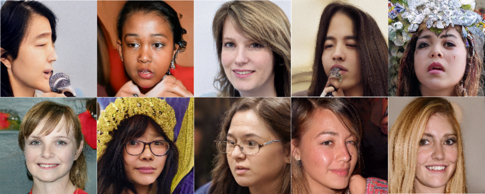
Here are some examples of faces which are generated by StyleGAN, starting from randomly sampled \(z\)s:

Now let’s take a look at \(w\). If we sample many \(z \sim Norm(0, I)\) and use \(f\) to map them to \(w\)-space, we see that although \(z\) is a standard isotropic Gaussian, \(w\) contains a lot of internal structure. \(w\) certainly is not normally distributed, and many features of \(w\) are correlated with each other.

Importantly, we’ll be (implicitly) leveraging this internal structure in \(w\) to generate Chernoff faces. In particular, for some data matrix \(X\), we’ll map each data point to some latent vector \(w\), and use \(w\) to generate a realistic-looking Chernoff face. Since we’re parameterizing the generation of a Chernoff face using a neural network, we completely evade the problem of relying on hand-engineered facial features, and we allow ourselves to (potentially) use the entire space of variation in faces (that have been learned by the model), not just the specific set of 18 features that someone has defined.

PCA and eigenspace projections

In order to map entries of \(X\) to \(w\), we can use PCA (principal components analysis). As a reminder, for some matrix of observations \(A\), PCA takes the (centered) covariance matrix \(\hat{A}\) and performs an eigendecomposition into \(\hat{A} = V\Lambda V^{T}\), where \(V\) contains the eigenvectors and \(\Lambda\) contains the eigenvalues. \(V^{T}\) maps objects to the eigenspace of \(\hat{A}\), \(\Lambda\) scales the entries according to the eigenvalues, and \(V\) transforms back.

Importantly, PCA identifies the most variable directions of the input space \(A\), and the matrix \(V\) interconverts between the input space \(A\) and the principal-components space (i.e. the eigenspace). In this principal-components space, the dimensions corresponding to the top principal components control the highest dimensions of variability in the input space \(A\).

We can apply PCA to our space of latent vectors, \(w\). Let us take a large sample of vectors \(w\), and collate them together into a big matrix \(W \in \mathbb{R}^{n\times 512}\). We perform PCA on \(W\).

Let’s explore the principal components of \(W\) a bit:

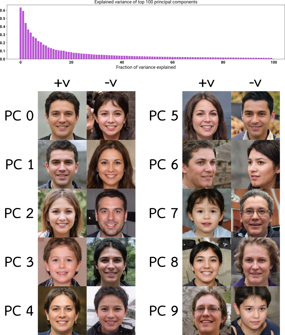
First off, the top 100 principal components (PCs) already explain a huge proportion of the variation in \(w\), which is nice to see. We can also show the faces generated by the eigenvectors of the top 10 PCs. This just shows the faces generated by eigenvectors of magnitude 1 (the choice of magnitude here is somewhat arbitrary). That is to say, for each of the top PCs, we take the eigenvector corresponding to that PC (of unit magnitude), and show the face generated by \(g\) in the positive and negative directions. Equivalently, we take a one-hot vector with a 1 or -1 in only one position, and use \(V\) to transform it from the eigenspace to \(w\)-space, and display the generated face.

In short, these are the axes of faces which correpond to the highest amount of variation in the latent space \(w\). It’s fun to try and figure out what sort of variation the model has picked up on for each PC. Several of them seem to capture notions of gender or age. Notably, PC 6 seems to correspond to the direction that the person is facing.

We can also verify that we can mix PCs and get some faces in between. Here is a selection of some mixed faces, where we take two PCs, and generate the face which corresponds to the mixing of the two. Here, for each PC, we have four combinations, which come from taking the positive or negative eigenvector for each PC:

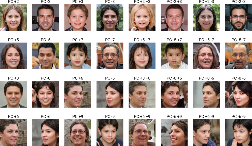
We can definitely see some nice mixes here, particularly with PC 6.

Algorithm for generating Chernoff faces

So here’s how we’ll actually use PCA to generate Chernoff faces:

We perform PCA on \(X\). This projects original data points into a lower-dimensional space of size \(d' \leq 512\).

At the same time, we’ll also perform PCA on \(W\), keeping the top \(d'\) principal components.

For each entry \(x\) in \(X\), we map \(x\) to the PC space of \(X\), and then we normalize the entries in PC space (dimension \(d'\)) by using a simple z-score transformation (i.e. subtract the mean and divide by the standard deviation, where the mean and standard deviation are computed empirically over a sample).

We then perform a reverse z-score transformation on this normalized PC-space vector, using the mean and standard deviation of the principal components of \(W\). This effectively aligns the PC-transformed \(x\)-space into PC-transformed \(w\)-space.

Finally, we use the eigendecomposition of \(W\) to transform back from \(w\)‘s PC space to \(w\)-space. The neural network \(g\) then maps this to an actual face image.

Examples of AI-generated Chernoff faces

Wine

Let’s start out with a toy example: the classic wine dataset which tabulates several features of a set of wines.

Here, we plot the top two PCs of the wine dataset, and show our generated Chernoff faces for a few points. We can see distinct faces for several extremes of the dataset in PC space. This is rather nice, because we are now able to visualize distinct faces for a dataset which would otherwise be too high-dimensional to visualize.

1000 Genomes

Now let’s move on to something even more challenging, and even more perverse. Let’s take the genomic variants (just on chr22 for simplicity) for the humans in the 1000 Genomes Project. Here, we have over 2500 individuals of 5 different superpopulations (Africans, Americans, East Asians, Europeans, and South Asians).

We can perform PCA on the variants, and we recover a very familiar plot:

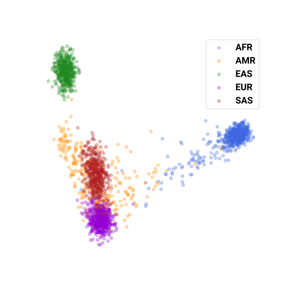
If we take the centroids of each superpopulation, we can apply our algorithm and transform it through PC space to \(w\) vectors, and generate faces for each of these superpopulations. This is what we get:

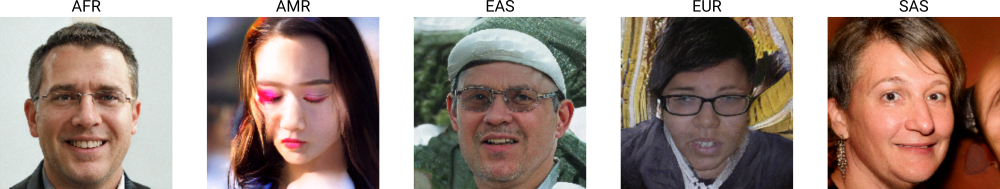
So these are the distinct faces which distinguish each superpopulation (on average). I swear I’m not an anarchist.

Limitations and future directions

Perhaps you’ve noticed that the faces we generate don’t look quite as diverse in terms of facial features and expressions compared to the cartoonish Chernoff faces from above or in other applications. This is almost certainly because StyleGAN is trained on facial datasets which typically only contain a single kind of expression, which is people smiling when posing for pictures. This severely limits the ability of our model to generate diverse faces of different expressions. Ideally, we would have a high-quality model which is trained to generate faces of many diverse expressions.

Even if we had such a model, however, there’s no guarantee that the model would identify axes of the most variability in the same way that humans do. For example, in the extreme, a model might use the background of the image or a person’s clothing (or some other minor detail) as a major principal component, and not features which we would rely upon for distinguishing faces (e.g. mouth expression). Further work would be needed in this area to better align a model’s major axes of variation with what we expect for Chernoff faces.

Reproducibility

The StyleGAN architecture and model weights were downloaded from Kim Seonghyeon’s GitHub repository (specifically, the weights for the 1024px-resolution model).

All code used to generate the results and figures in this post can be found in this Jupyter notebook.

1000 Genomes variants were downloaded from the online portal (phase 3).